User Documentation

Installation

When available, go to the download page and install Graphica3D. The setup file will take you through the setup process. And once done, run the application. You will then be asked to enter your license key - this will require an internet connection. And once done, you'll have full access to Graphica3D.

Using Graphica3D

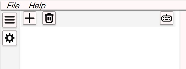
to add an input, press the plus button. This will create an input where you can add text. If you want to delete an input, hover over the input and click the button on the right hand side then click delete. Or if you want to delete all inputs, press the button with the trash can icon.

Function Types

1-d Scalar Functions

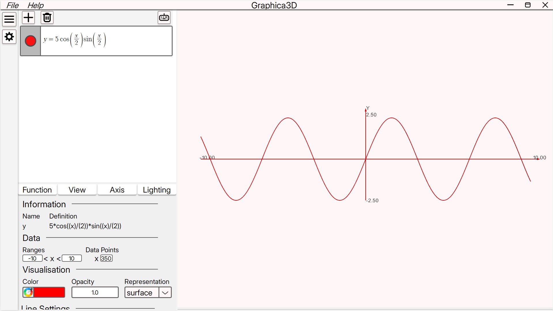
if you want to draw a 1-d scalar function, you can write either y = or f(x) =, then your function of choice. For function notation any name and any variable is allowed e.g valid functions for 2d scalar plots include g(x), l(t), hello(a), curve(s) etc. As long as the functions dependant variable in use does not match a user defined variable (which we will get too soon).

2-d Scalar Functions

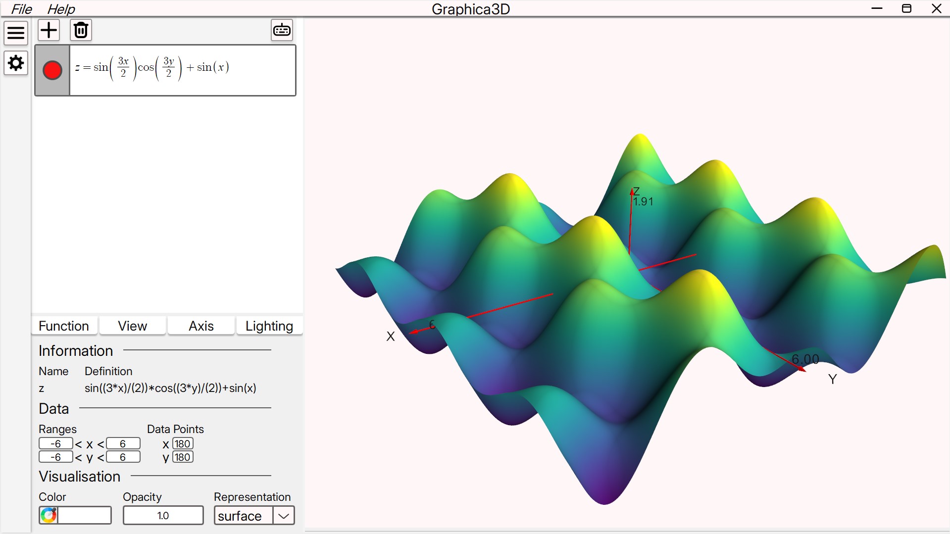
The other functions that can be drawn include 2-d scalar functions, which require two input variables. And are inputted as either z=, or f(x, y). Where again the name can be any text and the variables can be any, except the same as each other. e.g g(a, b), land(x, y) etc.

3-d Scalar Functions

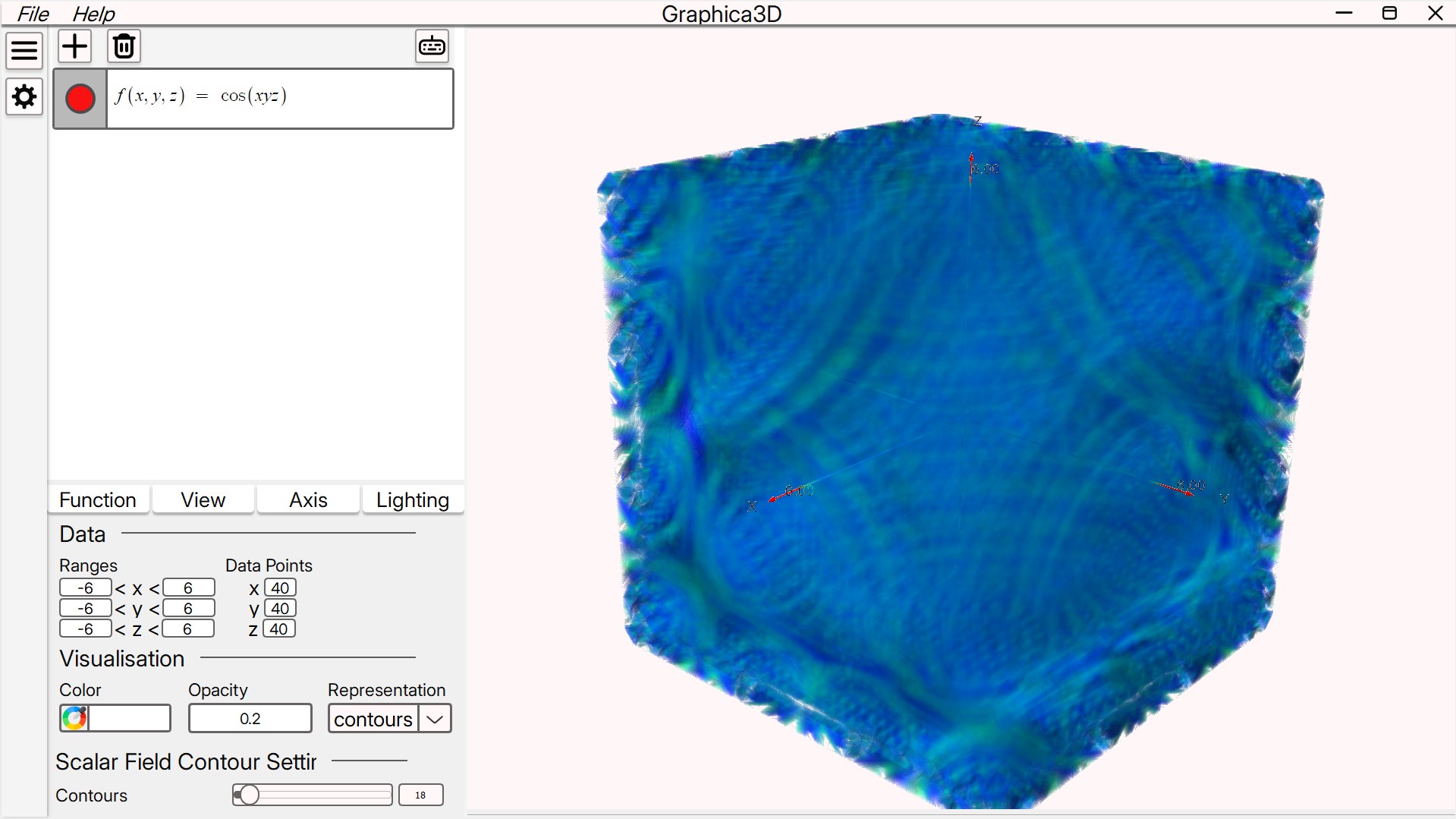
3-d scalar functions are very similar, except they require 3 input variables, and the notation follows the same rules. e.g f(x, y, z), scal(u, o, q) etc.

They can be customized by going to settings and going to the function tab, scrolling down allows two representation modes, contour plot and plane cut

The contour plot draws surfaces where the function is constant e.g for f(x, y ,z) = x*y*z, it may draw 12 contours which are 1 = x*y*z, 2 = x*y*z, etc. The number of contours can be adjusted

The slice plane representation creates a cut plane widget which can be dragged across the screen, showing via a colormap, how the scalar field varies in that space. The slice index, and orientation can be adjusted.

2-d Vector Fields

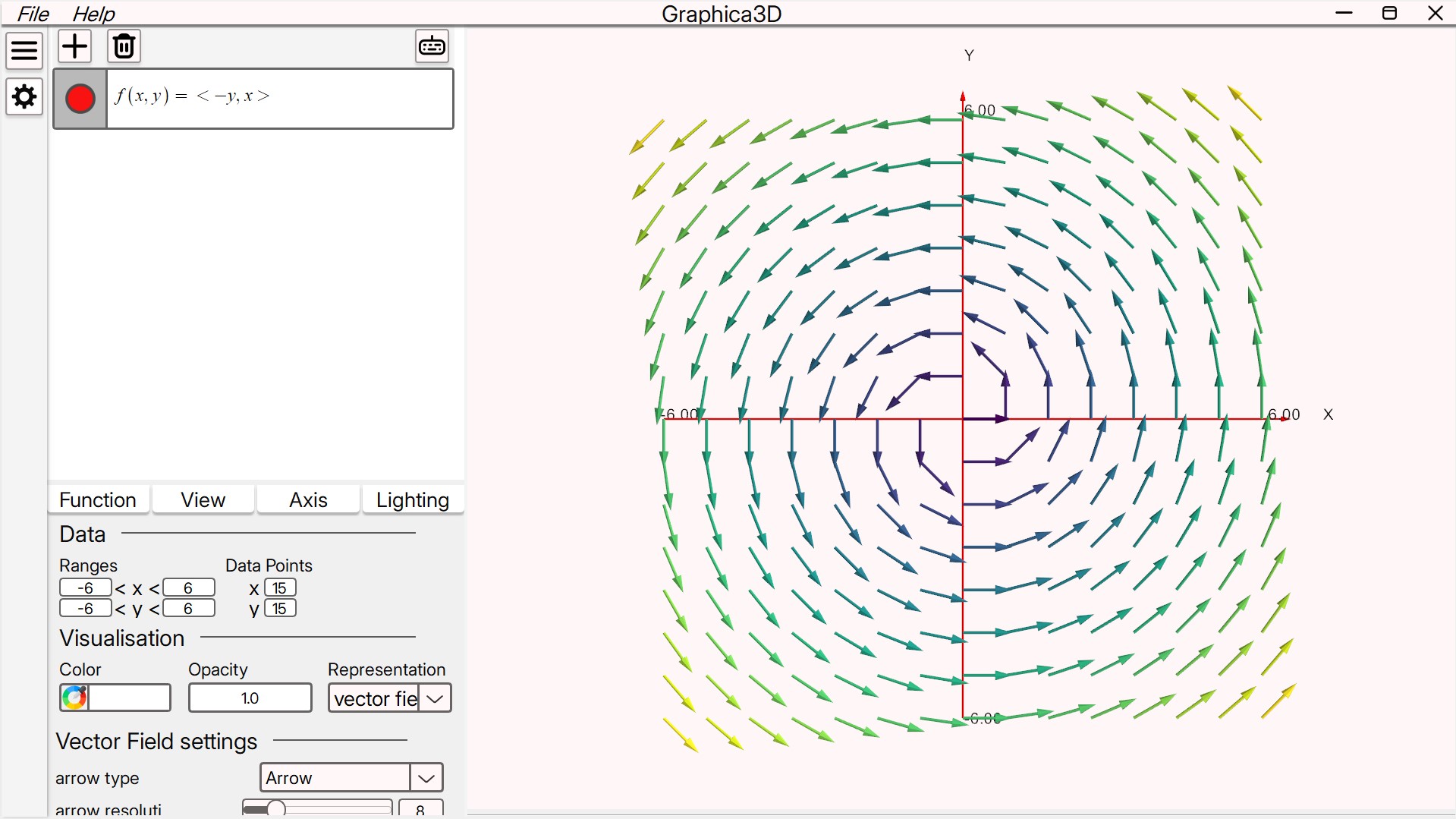
2-d vector fields take in 2 variables and output two functions, the notation required is in the form f(x, y) = <function, function>, where f can be any name and x, y can be any two independant variables some examples include f(x,y) = <x, y>, vec(o, c) = <c^2, -y*c/2> etc.

They can be cusomized in the function settings tab and can be changed between vector field representation - where a vector / arrow is drawn at each point with its direction the same as the field at that point and a colormap representing the various magnitudes. And Flow - where at each source, the vector field is integrated showing a line from each source, can be seen as how a particle would move if it was in a certain fluid flow.

3-d Vector Fields

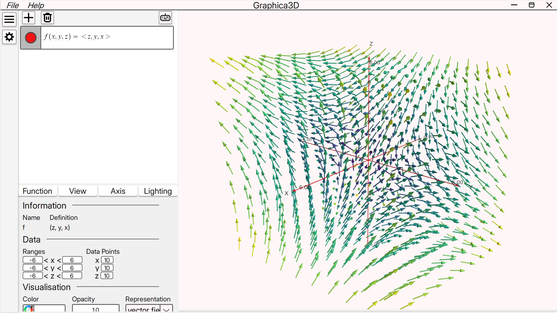
3-d vector fields are identical to 2-d except they take up another dimension. The notation is the same except one more input variable is required and one more output function is required. e.g f(x, y, z) = <function, function, function>. Where f can be any name, function is any function of the variables and the variables are all independant. They can be customized in the same way as 2-d, except the flow representaion is much more helpful.

2-d Parametric Functions

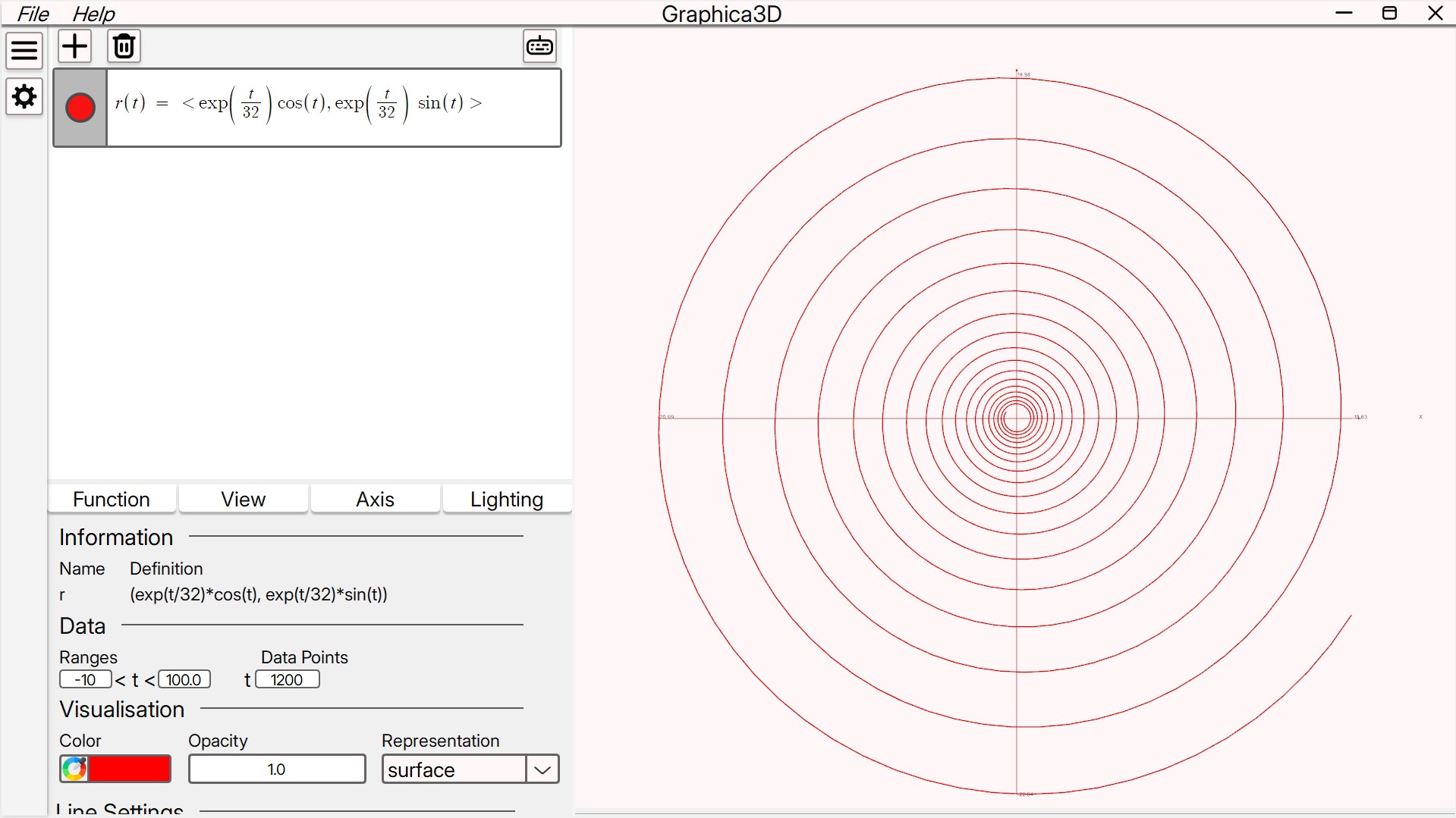
2-d parametric functions only take in one input variable, but have two output functions. The notation is f(t) = <function, function>. some example functions include: f(t) = <cos(t), sin(t)>, kl(p) = <p, tanh(p)> .

3-d Parametric Functions

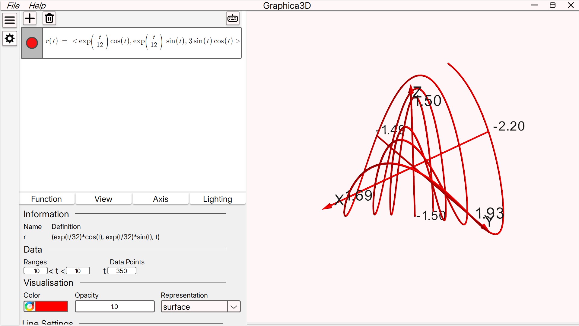
3-d parametric functions take in one variable and output three. They are just like 2-d except are shown in 3 dimensions. The notation is f(t) = <function, function, function>. Some example functions include: f(t) = <cos(t), sin(t), t>, kl(p) = <cos(p), tanh(p), 2p> .

Surface Functions

3-d surface functions are parameterised surfaces that take in two variables and output three functions. The notation is f(s, t) = <function, function, function>. Some example functions include: f(a, b) = <a*b, 2sin(a), cos(b)>.

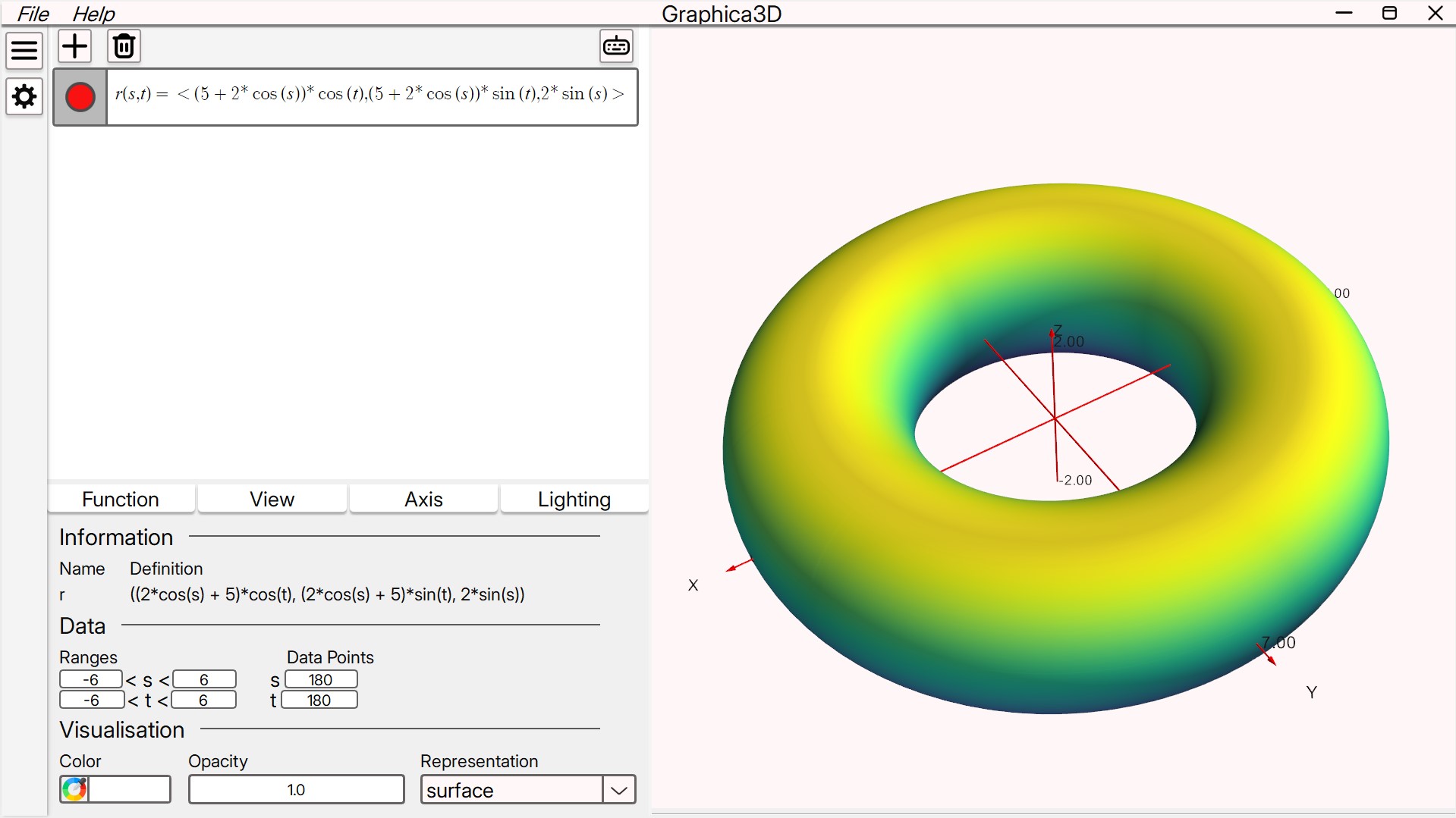
Customization of functions

once youve drawn a function on screen, there'll be an option to customize properties of how that function is rendered on screen. By going to either the settings button or clicking on the three dots that show up when hovering over the screen. Then you can press the settings option.

From here you can change the ranges of each of the variables, and the number of data points. More data points will improve the quality of the plot, but will reduce performance, especially if you plan on using variables to dynamically adjust how a plot looks over time.

Below that, you can change the color of the function. You can choose from a plain color or a colormap. A colormap will vary the color across the function dependant on the color scheme youve picked and dependant on the function type. The opacity of the plot can be changed, the value must be between 0 and 1 where 1 is opaque and 0 is invisible. The representation of a plot can too be changed different function types have different optional representations, some basic ones include wireframe and points.

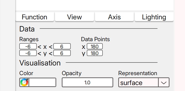
Then there's the custom function settings dependant on the function type. Certain function types have more customization options than others, for example 3d-scalar plots if in the contours representation will only have the number of contours option, while vector fields in flow representation have around 8 seperate properties that can be adjusted.

View Options

In the settings widget, there's a view tab. This allows you to adjust the viewing mode, along with changing the camera properties for any fine tuning.

viewing modes - Graphica3D supports two viewing modes, crop mode and scale mode. Crop mode creates an invisible grid around the focal point and only shows data within that grid. For example, if you have a 1d scalar function y=100x, with ranges -6<x>6, but the focal point is at (0, 0) and crop mode is enabled then the max y value shown is 12, so the function cuts off at x = 0.12. But you can zoom out, which will show more of the function. Crop mode is useful for navigating functions, especially in 3d trying to explore them and find interesting areas of them. Crop mode only affects 1-d, 2-d scalar functions and 2-d vector fields.

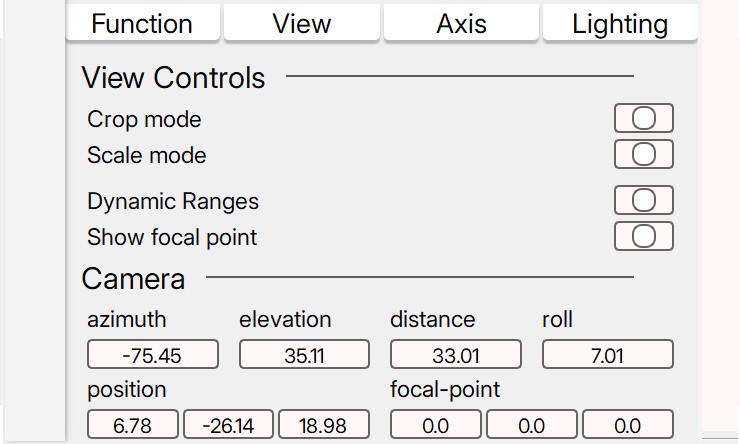
Scale mode adjusts either the z or y value to fit within a cube shape. Say if we have our same function y=100x, with the same ranges -6 and 6, the y scale will be appropriatley scaled down so that y=600 is shown as the maximum but physically on screen its the same length as the x axes.

camera properties - this option allows you to change the position of the camera.

Axes options

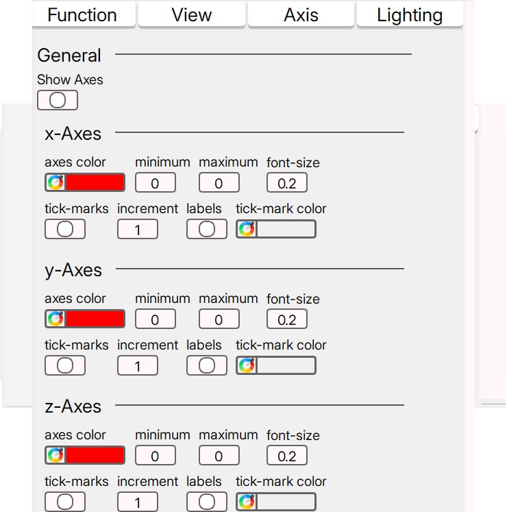
the axes options allows you to toggle the axes on or off, having the axes off improves perfomance, but having it on can be very helpful. Each axis in each dimension can be adjusted individually, the font size and color can be adjusted. And the option for tick marks and labels is available along with the tick increment option.

Lighting options

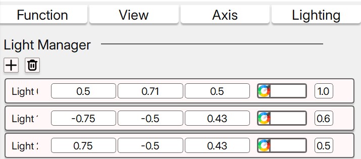
In the lighting tab, you can add lights into the scene and take them away. The position, color and intensity can all be adjusted. Graphica3D allows for up to 64 lights on screen.

Variables

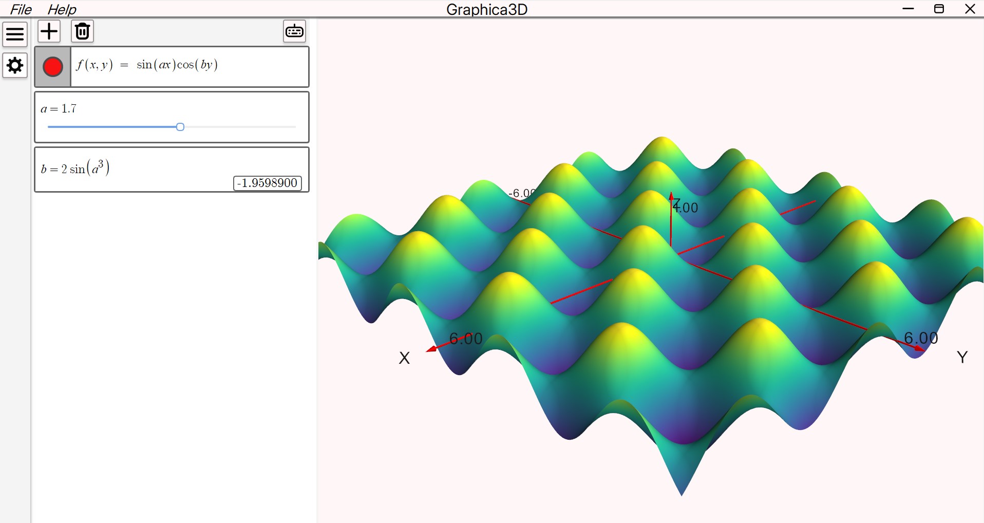
You can define variables in an input, by typing the name of the variable then what it's equal to, for example a=1, or b=10. Then a slider will show on screen where you can adjust the value. Variables can be used in equations, and if a variables value is changed, the functions that use it will dynamically update. For better performance turn off the axes. Variables can also be defined by setting them equal to an expression e.g c = sin(2+\sqrt(a)), (as long as 'a' is defined previously).

File Saving

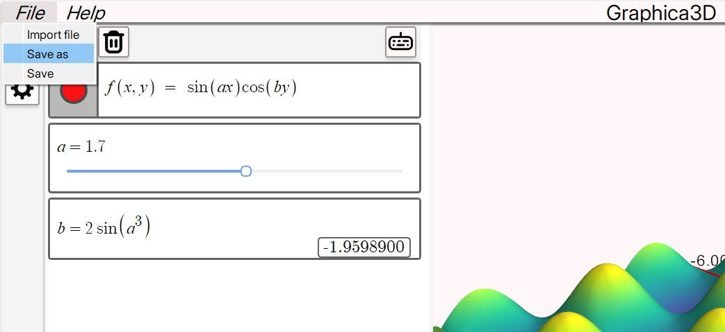
Files can be saved by going to the file menu option and pressing save as. A JSON file will be saved in the place that you want it to, and can be imported whenever. Importing a file wipes the current data in Graphica3D.

Other

This software is in beta and in it's very early stages. More features will come out in future updates along with bug fixes and performance improvements. If you have any queries, want to report a bug or need to contact us. Send us a message here.